Working with Python packages

This page is the third post in a series of introductory python tutorials:
1. Installing Python using Conda
2. Getting started with Jupyter
3. Using Python packages - this tutorial
4. Working with data
5. Making figures in Python

Python is a powerful language, however, the real strength of the Python environment comes from the open-source community that has written 1000s of packages to make certain tasks easier.

Eventually, we will cover how to write your own packages to better organize your own code or share your work, but this tutorial will focus on introducing some of the most widely used packages in scientific research. This is not meant to be a comprehensive review of the Python ecosystem but rather a high-level overview to provide a flavor of different packages.

Installing Python Packages

There are several methods for installing Python packages. In our tutorials, we will use Conda as our default package manager due to it’s relative ease of use. For packages that aren’t on Conda, we suggest using pip to install from the Python Package Index (PyPI).

Conda is a non-python specific package manager

Notes:

• Conda installs from binaries and is much better at handling non-Python dependencies than pip

Examples:

conda install scipy

conda list --export > package-list.txt

PyPI and pip

PyPI is the Python Package Index - an open repository that anyone can submit a package to.

Notes:

• We can use pip to install packages from PyPI and use them in our own code.
• pip installs packages from source (or from wheels) that are uploaded to PyPI.
• Pip is specific to Python code, which can make it difficult to install packages with non-Python dependencies (things that rely on C or Fortran code for example)

Examples:

pip install pandas
pip freeze > requirements.txt
pip install --upgrade pandas

Selected “popular” python packages

We won’t cover all of these in depth here, but here are a list of packages that tend to be useful in different settings

• Plotting: seaborn, matplotlib, bokeh
  
• Data Manipulation and numerical computing: numpy, scipy, pandas
• Machine learning: scikit-learn, TensorFlow, theano
  
• Image processing: scikit-image, Pillow
• Documentation and testing: Pytest, sphinx, unittest

Introduction to several packages with short examples

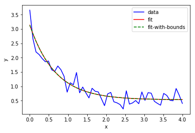
SciPy is a collection of open-source Python libraries for mathematics, science, and engineering

• Contains many useful tools for optimization, signal processing, curve fitting
• Tip: SciPy can be on the more difficult side to install due to all of the C dependencies. Highly recommended to use Conda as a package management tool
• Example:

import numpy as np
import matplotlib.pyplot as plt
from scipy.optimize import curve_fit

def func(x, a, b, c):
    return a * np.exp(-b * x) + c

# define the data to be fit with some noise

xdata = np.linspace(0, 4, 50)
y = func(xdata, 2.5, 1.3, 0.5)
y_noise = 0.2 * np.random.normal(size=xdata.size)
ydata = y + y_noise
plt.plot(xdata, ydata, 'b-', label='data')

# Fit for the parameters a, b, c of the function func

popt, pcov = curve_fit(func, xdata, ydata)
plt.plot(xdata, func(xdata, *popt), 'r-', label='fit')

# Constrain the optimization to the region of 0 < a < 3, 0 < b < 2 and 0 < c < 1:

popt, pcov = curve_fit(func, xdata, ydata, bounds=(0, [3., 2., 1.]))
plt.plot(xdata, func(xdata, *popt), 'g--', label='fit-with-bounds')

plt.xlabel('x')
plt.ylabel('y')
plt.legend()
plt.show()

NumPy a very useful library for scientific computing. It adds support for arrays, linear algebra tools and optimized integration with C/Fortran

• Used by many, many other numerical/scientific computing packages
• Potentially useful: NumPy for MATLAB users
• Example:

import numpy as np

x = np.linspace(0,10, num=10)
y = np.random.random(len(x))

y_mean = y.mean()
y_std = y.std()

print('Mean = {0:.3f} \t Std. Dev. = {1:.3f}'.format(y_mean, y_std))

plt.plot(x, y, 'o')
plt.ylim(0,1)
plt.show()

Python Data Analysis Library (http://pandas.pydata.org/)

• Amazingly useful library for importing, manipulating, cleaning data from a wide variety of sources
• Examples:

Easily read in data from csv, excel, json, etc.

Note: you can download the example file we use here

# import the pandas package
import pandas as pd

# read in the data from our file
data = pd.read_csv('./time-data(833).txt')

# assign names to each of the columns for easy reference
data.columns = ['time(s)', 'current(A)', 'potential(V)', 'frequency(Hz)', 'amplitude(A)']

# print out the first 5 rows of our data
data.head()

Manipulate data (remove columns with NaN, calculate mean, apply function to all rows)

# drop columns with NaN
data.dropna(axis=1)

#calculate mean
data["current(A)"].mean()

#calculate power directly
power1 = data["current(A)"]*data["potential(V)"]

# or apply lambda function row-by-row
power2 = data.apply(lambda x: x["current(A)"]*x["potential(V)"], axis=1)

# compare the two methods
(power1 == power2).all()

Easily save data

data["power(W)"] = power1

data.to_csv("./add_power.txt", index=False)

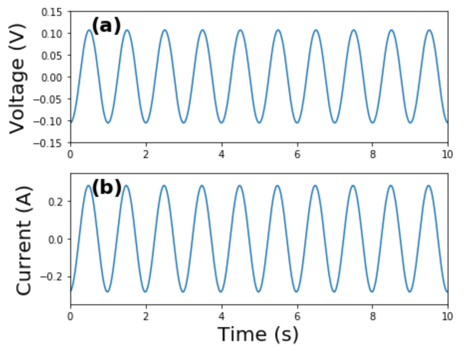
Matplotlib is a powerful Python plotting library and forms the basis for many other plotting libraries

• Simple to use simply, but a LOT of low-level control if you want it…
• Examples:

time = data["time(s)"]
voltage = data["potential(V)"]
current = data["current(A)"]

fig = plt.figure(figsize=(6.5,5))
ax1 = fig.add_subplot(211)
ax1.plot(time, voltage)
ax1.set_ylabel("Voltage (V)", fontsize=20)
plt.ylim(-.15,.15)

ax2 = fig.add_subplot(212)
ax2.plot(time, current)
ax2.set_ylabel("Current (A)", fontsize=20)
ax2.set_xlabel("Time (s)", fontsize=20)
plt.ylim(-.35,.35)

labels = ['(a)', '(b)']
for i, ax in enumerate([ax1, ax2]):
    ax.set_xlim(0,10)
    ax.text(.055, .85,labels[i], transform=ax.transAxes, fontsize=20, fontweight='bold')

plt.tight_layout()
plt.show()

fig.savefig('./example_plotting.png', dpi=300, bbox_inches="tight")

Seaborn is a high-level library for plotting many different statistical plots

https://seaborn.pydata.org/examples/index.html

import numpy as np
from scipy import stats
import matplotlib.pyplot as plt
import seaborn as sns

sns.set(color_codes=True)

x = np.random.gamma(6, size=200)
sns.distplot(x, kde=False, fit=stats.gamma)
plt.show()

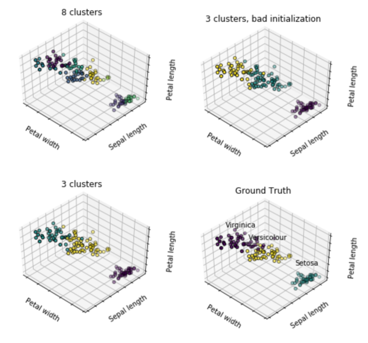
scikit-learn is machine learning in Python

• Example:

# Code source: Gaël Varoquaux
# Modified for documentation by Jaques Grobler
# License: BSD 3 clause

import numpy as np
import matplotlib.pyplot as plt
from mpl_toolkits.mplot3d import Axes3D

from sklearn.cluster import KMeans
from sklearn import datasets

np.random.seed(5)

iris = datasets.load_iris()
X = iris.data
y = iris.target

estimators = [('k_means_iris_8', KMeans(n_clusters=8)),
              ('k_means_iris_3', KMeans(n_clusters=3)),
              ('k_means_iris_bad_init', KMeans(n_clusters=3, n_init=1,
                                               init='random'))]

fignum = 1
titles = ['8 clusters', '3 clusters', '3 clusters, bad initialization']
for name, est in estimators:
    fig = plt.figure(fignum, figsize=(4, 3))
    ax = Axes3D(fig, rect=[0, 0, .95, 1], elev=48, azim=134)
    est.fit(X)
    labels = est.labels_

    ax.scatter(X[:, 3], X[:, 0], X[:, 2],
               c=labels.astype(np.float), edgecolor='k')

    ax.w_xaxis.set_ticklabels([])
    ax.w_yaxis.set_ticklabels([])
    ax.w_zaxis.set_ticklabels([])
    ax.set_xlabel('Petal width')
    ax.set_ylabel('Sepal length')
    ax.set_zlabel('Petal length')
    ax.set_title(titles[fignum - 1])
    ax.dist = 12
    fignum = fignum + 1

# Plot the ground truth
fig = plt.figure(fignum, figsize=(4, 3))
ax = Axes3D(fig, rect=[0, 0, .95, 1], elev=48, azim=134)

for name, label in [('Setosa', 0),
                    ('Versicolour', 1),
                    ('Virginica', 2)]:
    ax.text3D(X[y == label, 3].mean(),
              X[y == label, 0].mean(),
              X[y == label, 2].mean() + 2, name,
              horizontalalignment='center',
              bbox=dict(alpha=.2, edgecolor='w', facecolor='w'))

y = np.choose(y, [1, 2, 0]).astype(np.float)
ax.scatter(X[:, 3], X[:, 0], X[:, 2], c=y, edgecolor='k')

ax.w_xaxis.set_ticklabels([])
ax.w_yaxis.set_ticklabels([])
ax.w_zaxis.set_ticklabels([])
ax.set_xlabel('Petal width')
ax.set_ylabel('Sepal length')
ax.set_zlabel('Petal length')
ax.set_title('Ground Truth')
ax.dist = 12

fig.show()