By Matt Murbach
This page is the second post in a series of introductory python tutorials:
1. Installing Python using Conda
2. Getting started with Jupyter - this tutorial
3. Using Python packages
4. Working with data
5. Making figures in Python
Jupyter is an open-source web application allowing you to run “notebooks” in your browser. These notebooks can contain code, equations, and visualizations in one, interactive, and shareable place.
If you want to quickly demo the notebooks online you can go to https://try.jupyter.org/
In this post, we will discuss installing Jupyter and demo some of the useful features of this technology. A Jupyter notebook with the below examples can be downloaded here: intro-to-jupyter.ipynb
1. Installing Jupyter
Installing Jupyter and Jupyter Lab
Open your command prompt or Git BASH (Windows) or a terminal (OS X, linux)
- Install Jupyter by running
conda install jupyter notebook - Install Jupyter Lab by running
conda install -c conda-forge jupyterlab
2. Running the Jupyter application
Navigate to the directory you’d like to work in
Run the following in your command prompt or terminal to create a directory in your Documents folder for this tutorial.
Note: the cd command means change directory and mkdir makes a directory
(Command prompt)
C:\Users\your-username> cd ~/Documents/
C:\Users\your-username\Documents> mkdir jupyter-tutorial
C:\Users\your-username\Documents> cd jupyter-tutorial
C:\Users\your-username\Documents\jupyter-tutorial>
Opening Jupyter Lab
To open the application simply run the command jupyter lab
C:\Users\your-username\Documents\jupyter-tutorial> jupyter lab
A few seconds after executing the above code, your default browser should open and you should see:

3. Creating a new notebook
To create a new notebook, click on “Python 3” under the notebook header:
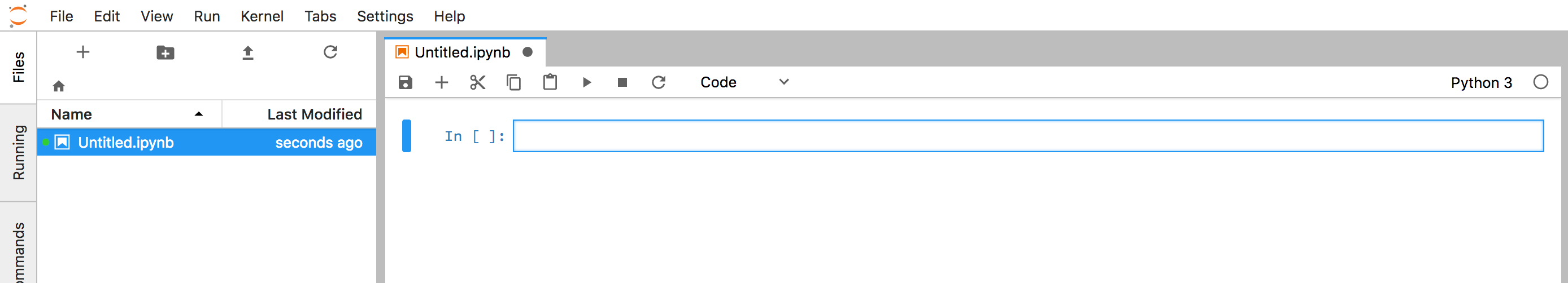
which will create a blank notebook document titled “Untitled.ipynb” that is now displayed as a tab:
4. Overview of notebook components
Before we start writing code, let’s take a second to explore the notebook itself:
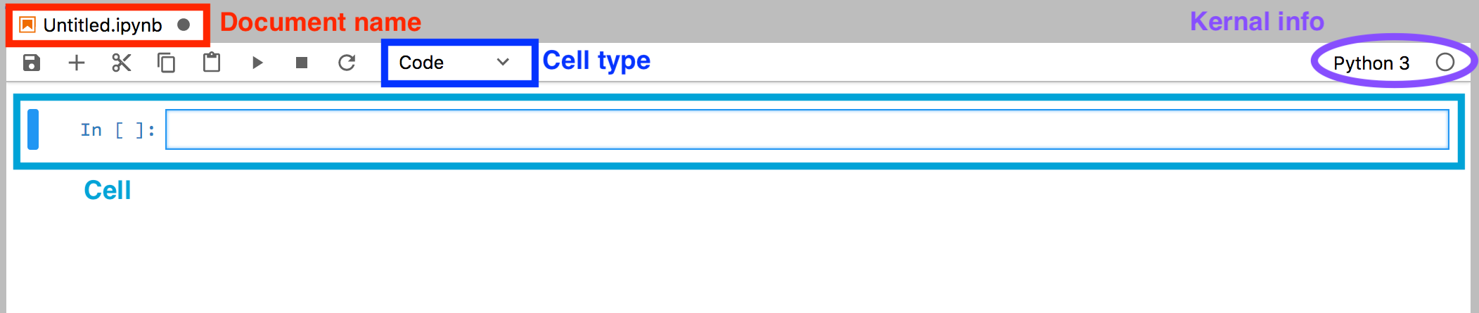
- To change the filename, simply right-click on the title and rename the file
- We can see that the kernal here is a Python 3 kernal and that it is currently not executing anything (dot is unfilled)
- We will put the cell type selection into good use below to switch between code and markdown
5. Let’s execute some code!
Let’s start by typing some example Python code into the cell:
import datetime

hackWeek = datetime.date(2018, 5, 14)
now = datetime.datetime.now().date()

print('There are {} days left until the ECS Hack Week. Get stoked!'.format((hackWeek - now).days))
To execute this cell we can press shift + enter
6. Modularity makes it easy to develop code in bite size chunks
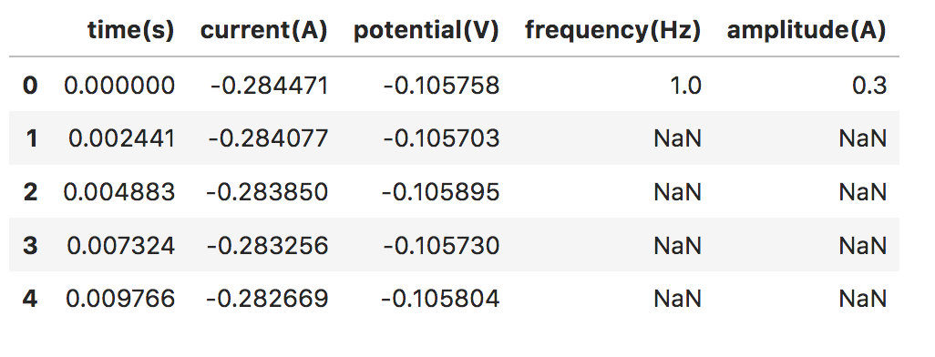
Step 1. Data intensive operation
# import the pandas package
import pandas as pd

# read in the data from our file
file_location = 'https://raw.githubusercontent.com/mdmurbach/ECS-Hack-Day-2017/master/time-data(833).txt?raw=true'
data = pd.read_csv(file_location)

# assign names to each of the columns for easy reference
data.columns = ['time(s)', 'current(A)', 'potential(V)', 'frequency(Hz)', 'amplitude(A)']

# print out the first 5 rows of our data
data.head()
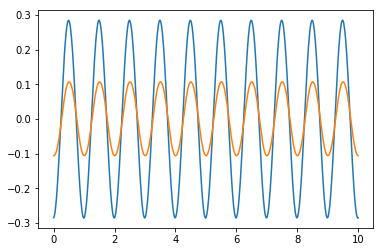
Step 2. Visualization or exploratory data analysis
# import the matplotlib package
import matplotlib.pyplot as plt

# plot the current and voltage vs time
plt.plot(data['time(s)'], data['current(A)'])
plt.plot(data['time(s)'], data['potential(V)'])

plt.show()
7. Other cool features:
In addition to running code snippets in cells, Jupyter also has several other handy features.
Markdown
Jupyter cells can also be used to display equations, documentation, and tables using Markdown.
To demonstrate this, click on a new cell and select ‘Markdown’ from the cell type dropdown menu at the top of the notebook.
Type some Markdown:
### Lists
- a
- b

### Equations
$$
\frac{\partial (\epsilon c)}{\partial t} = \frac{\partial}{\partial x}\left( \epsilon D_{eff}\frac{\partial c}{\partial x} \right) + a (1-t_+^0) j_n
$$

### Tables

| Name | | Column |
|:---:|:---:|:---:|
||This is a fun table||
|To Do| Fill in the rest| |
and click shift + enter again to execute the cell. This time instead of executing code, you should see the following display:
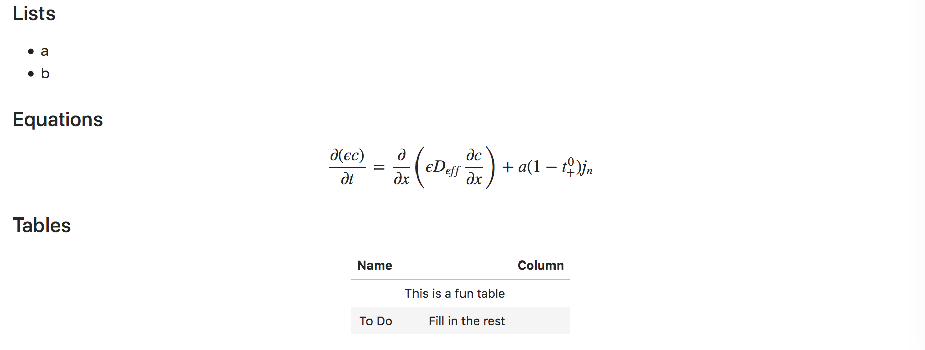
Markdown is a powerful tool to display images/equations/code/notes easily (all the tutorial posts here are written in Markdown for example). For additional information on Markdown syntax, there are several ‘Markdown Cheatsheets’ (e.g. here or here) or an interactive markdown editor to explore with.
Keyboard shortcuts
Just like we used the shift + enter shortcut to execute a cell, there are lots of other shortcuts which make it even easier to work within Jupyter notebooks.
There are two different ‘modes’ you can be in when using the notebook (Command mode and Edit mode).
You can tell which mode based off of the color of the cell outline (blue = Command mode, green = Edit mode) and you can switch between the two using the esc and enter keys.
For example,
- Click on a cell so you can type code (you’re now in edit mode)
- Push
esc(to switch to Command mode) - Push
b(this is the shortcut to create a new cell below your current location) - Push
m(to switch this cell type to Markdown) - Push
enter(to enter Edit mode) - Type some Markdown code
- Use
shift+enterto execute
Here are a few useful shortcuts (you can see all of them by hitting h in command mode):
Useful command mode shortcuts
| Command | Action |
|---|---|
| a | Create new cell above |
| b | Create new cell below |
| d d | Delete current cell |
| z | Undo delete cell |
| m | Change cell to markdown |
| y | Change cell to code |
| h | Bring up the list of shortcuts |
Useful editing shortcuts
| Command | Action |
|---|---|
| Ctrl-a | Select all |
| Ctrl-c | Copy |
| Ctrl-v | Paste |
| Ctrl-s | Save |
| Tab | Autocomplete |
| Shift-tab | Tooltips |
Support for lot’s of different languages
While Jupyter grew out of IPython and stands for Ju (Julia) + py (Python) + r ( R ), the Jupyter environment supports kernals for many many (~75) other languages
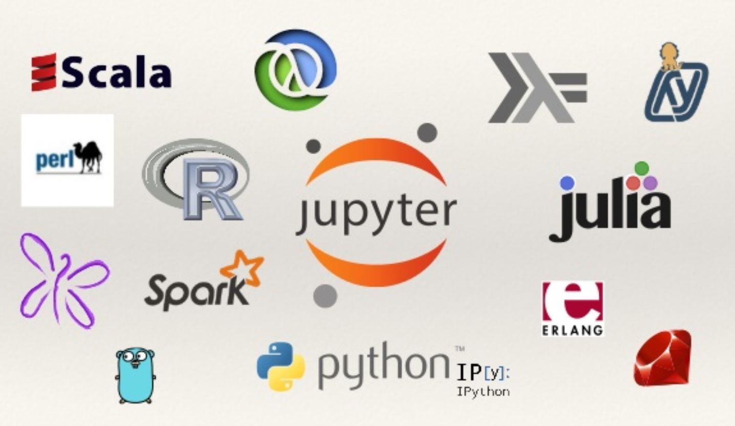
Image from Fernando Perez PLOTCON talk
If you’ve made it this far, congratulations!
You now have Jupyter installed and know your basic way around using notebooks for executing code and displaying Markdown. In the next tutorial, we’ll introduce several useful Python packages and start performing some more useful analysis. Part 3. Using Python packages.